The letter ‘P’: small in size but great in spirit
Understanding the science of data
This article was published in MedinLux and is part of a collaborative effort to make statistical and epidemiological concepts accessible to healthcare professionals in Luxembourg.
This article is the first in the series on statistical methodology, providing tools to better understand and interpret scientific articles. The goal is to develop critical thinking and to get to know the best practices to follow when reading scientific information (or when analyzing your own data). In biomedical research, it is common to read “statistically different” or “significantly larger/smaller”, to see tables with a column where the letter “p” appears, or to see graphs containing stars (or other symbols). All of these refer to the same idea: the p-vaalue (probability value). However, what does it actually mean? In this article, we will present it to you in more details
AN EXAMPLE FROM THE LITERATURE TO ILLUSTRATE OUR POINT
In a scientific article from 2021, the authors studied the birth weight of babies with reference to the smoking habits of the mothers (1), taking into account the mothers’ body mass index (BMI). The data were from a German perinatal survey and concerned more than 110,000 pregnancies, happening in the period between 2010 and 2017. The abstract indicated that the differences in babies’ weight between smokers and non-smokers were always statistically significant (p < 0.001), regardless of the mother’s BMI.
Let’s put ourselves in the shoes of the research team and ask the questions they must have asked. The team’s objective was to analyze the relationship between smoking and birth weight, taking into account maternal BMI. Figure 1 shows the different steps from defining the research hypothesis to the conclusions.

FIRST, DEFINE THE HYPOTHESIS
In research, the hypothetic deductive approach aims to explicitly define a null hypothesis and an alternative hypothesis. The null hypothesis is formulated, so that it can be rejected. It is considered true until the contrary is demonstrated. Conversely, the alternative hypothesis is the one we seek to demonstrate evidence for. They are mutually exclusive: both of them can never be true at the same time.
In our example, the null hypothesis is “there is no difference in weight between babies, whether the mother smokes or not”, while the alternative hypothesis can be stated as follows: “a difference in birth weight exists between babies of smokers and non-smokers”.
In practice, the decision is based on rejecting or not rejecting the null hypothesis, keeping in mind that we wish to find evidence for the alternative hypothesis. Thus, scientists use statistical tests to determine whether the null hypothesis is true or false. If they can demonstrate with a certain probability that the null hypothesis is false, then the alternative hypothesis will be “accepted” (2).
SET THE LEVEL OF UNCERTAINTY
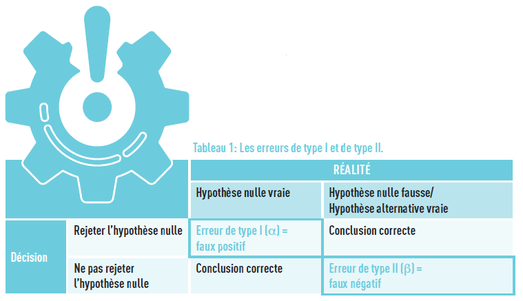
Once the hypotheses are clearly stated, we focus on the level of uncertainty, that is, the level of risk of error we are willing to have in rejecting the null hypothesis (and thus “accepting” the alternative hypothesis) when it is actually true. This is the risk of a Type I error, the risk of a “false positive” result, denoted by α. It is chosen according to the field and the stakes of the study. Generally, it is set at 5% (two-sided, i.e., there is a difference in either direction, with 2.5% chance at each side). This means that if the experiment is conducted 100 times (on different samples, for example), the null hypothesis will be rejected 5 times when it is actually true.
REMARK FROM THE STATISTICIAN
The 5% threshold is not randomly chosen. This limit is derived from a normal distribution (also known as the Laplace-Gaussian distribution, the famous bell-shaped curve; an absolute reference among statisticians, it corresponds to the distribution of many biological variables): when values are more than two standard deviations away (in the case of a normal distribution with a Type I error of 5%, the threshold is 1.96) from the mean, they are considered unusual (3). The statistician may seek to minimize this risk by choosing, for example, a 1% threshold instead of 5%, which would make it more difficult to reject the null hypothesis, but would decrease the chance of false positive results
Another error to consider is the “false positive”. During a statistical hypothesis test, it is possible to accept the null hypothesis when it is actually false, known as a Type II error, denoted as β. In our example, this would mean concluding that babies have the same weight regardless of whether their mother smokes or not (when in fact they have different weight). This chance of error is used in calculating the power of the test (1 – β), which represents the probability of rejecting the null hypothesis when it is false.
These two errors are related: when one is reduced, the other will increase, and vice versa. Table 1 below summarizes the situations.
FORMING THE STUDY POPULATION
Before embarking on a study, it is important to determine the number of participants to include. Why go through this process? It is to avoid recruiting too many patients, which may incur significant costs and/or time, or could cause ethical issues in the case of interventional studies (exposure to potentially ineffective or even dangerous treatments). Conversely, a sample size that is too small would not provide sufficient power and would not lead to a conclusive result, leading to a false negative.
Several pieces of information are necessary to determine this number: the size of the targeted effect (based on historical data, existing research or researchers’ expectations), the power, Type I error rate, data variance, and the statistical test or model used during the analysis.
Additionally, the sample must be representative of the target population we wish to study, sharing a range of important properties with it. Thus, the sample should represent the characteristics of the target population, such as the same proportion of women/men, average age, etc. Without this, the results obtained in the study cannot be generalized.
In the example chosen, the authors sought data on babies and the smoking status of mothers (and mothers’ BMI).
COLLECTING THE DATA
Once all of that has been established a priori, the data can be collected.
In our example, the researchers used a large database (from the province of Schleswig-Holstein) that was part of the German Perinatal Survey, including 110,047 unique pregnancies recorded between 2010 and 2017. This study is therefore a registry-based study (we will later revisit the different types of studies, with their advantages, disadvantages, and limitations), with a considerable sample size (which ensures statistical power, as discussed earlier).
After data collection, various indicators specified in the protocol will be calculated to address the research question (such as the mean of a parameter across different groups, odds ratio, relative risk, etc.). These concepts will be explored in a forthcoming article.
Returning to our example, the researchers calculated the average birth weight of babies in the smoking group and in the non-smoking group, and compared these figures, while accounting for the mother’s BMI during pregnancy.
CALCULATING THE TEST STATISTIC AND DETERMINING THE P-VALUE
The fundamental question at this stage is whether the difference observed in our indicator — the birth weight of babies in smoker and non-smoker mothers — is related to the smoking status or is observed due to a random chance. To answer this question, statistical tests are employed, such as tests of means or medians, or even the Chi-square test, to name a few well-known ones, which provide the famous p-value. However, a statistician will always be invaluable in advising on which test is most appropriate for your research.
The p-value is a probability and therefore ranges between 0 and 1 (0% to 100% chance). The smaller the p-value, the stronger the evidence against the null hypothesis. It is then compared to the previously selected Type I error rate, α.
If the p-value is smaller than α, the results are considered statistically significant, and the null hypothesis is rejected with a risk of a false positive of α. Conversely, if the p-value is larger than α, the null hypothesis is not rejected.
REMARK FROM THE STATISTICIAN
In the interests of good practice, it is strongly recommended to report the numeric p-value as well, rather than only using symbols like stars in a graph or stating “< 0.05” in text or tables!
In our example, birth weight was highest among non-smokers. In all maternal BMI groups, birth weight significantly decreased with the number of cigarettes smoked per day (p < 0.001). In other words, chance has less than 1 in 1,000 experiments of explaining the observed difference
THE CONFIDENCE INTERVAL: ANOTHER INDICATOR, WITH MANY ADVANTAGES
The confidence interval (CI) provides more information than a single p-value: it presents the range within which will lie the estimated parameter in 95% of experiments (corresponding to a 5% risk). This means that if we were to estimate the effect 100 times (100 replicates of the study, i.e. population sampled 100 times), the parameter would fall within the interval in 95 out of 100 experiments.
Moreover, conclusions regarding statistical significance can also be drawn based on the CI. Referring back to the introductory example, if the odds ratio (a measure of the association) between having a prematurely born baby and the mother’s smoking status is calculated, and the value 1 is not within the interval, which indicates a statistically significant effect between these variables at a 5% risk level.
An important advantage of the CI is its ability to account for measurement variability. If the interval is wide, the estimation is less precise compared to when it is narrower.
REMARK FROM THE STATISTICIAN – FALSE POSITIVE AND NEED FOR CORRECTION MULTIPLE TESTS
A complication arises with the use of p-values when multiple tests are conducted on the same sample. Let’s revisit the example of studying the effect of tobacco on baby weight and imagine that the authors also want to test the effects of taking certain medications, different levels of physical activity, consumption of fruits and vegetables, home renovation activities (in preparation for the baby’s arrival), and stress during pregnancy. By definition, if there 5 are conducted with a 5% significance level each, the overall chance of false positive results multiplies with each added comparison, resulting in an overall significant level much larger than 5%.
To draw a parallel with justice, Type I error corresponds to convicting someone guilty when he/she has not committed the crime, and Type II error is to judge someone innocent when he/she has committed the crime
REMARK FROM THE STATISTICIAN – DATA CRUNCHING
Some researchers approach things incorrectly, even if it is not done intentionally. Instead of testing a hypothesis, but potentially facing pressure to publish, they go fishing for statistical associations. This practice is known by several terms: p-hacking, data dredging, data fishing, data snooping, or data butchery. It can take various forms: conducting analyses until finding results with a p-value below a certain threshold (usually 0.05), changing the evaluation criterion, using a restricted dataset with a population different from the original (e.g. excluding participants, or only considering a specific category of the population), using multiple/other adjustment variables (or ignoring some), and only showing significant tests (publication bias). By removing non-significant tests, the likelihood of showing significant results increases. Not using correction for multiple tests is a way to alter results, given that some results might be significant purely by chance.
More and more journals are becoming aware of these issues: they now require the publication of data to replicate analyses and verify published results. The best practice is to write a statistical analysis plan in advance, describing the different analyses, hypotheses, and proposed solutions, always with the support of a statistician.
THE CONTROVERSY OF THE P-VALUE
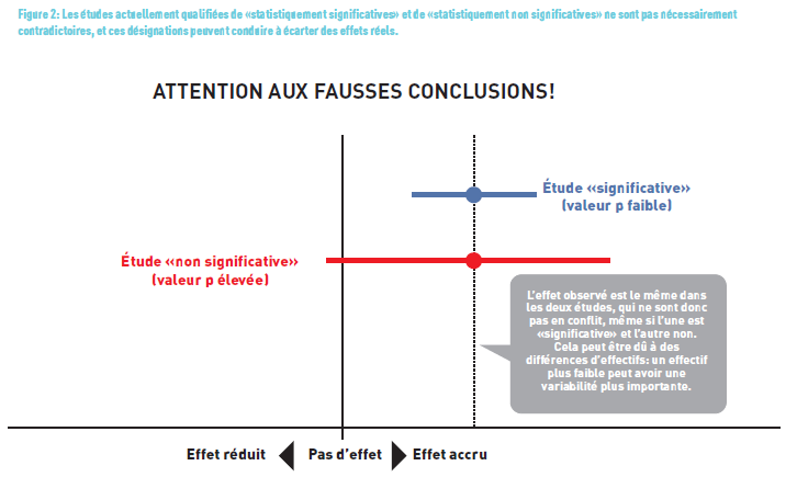
In recent years (even decades), many statisticians have criticized the use of p-value, notably in an article published in Nature (4) (Figure 2). In this article, the authors highlighted that 51% of the 791 articles across five journals had misinterpreted the p-value. They advocate against dichotomizing it into “statistically significant” or “not statistically significant” for decision-making purposes. The “p-value” should not be judged in isolation but rather placed in context, remembering that statistical significance is different from clinical significance.
TAKE HOME MESSAGE
The p-value — commonly referred to as “little p” — is a standard of scientific articles, even though its interpretation can be erroneous. However, by applying certain rules, it is possible to avoid the pitfalls discussed in this article or even provide a better understanding of estimates using CI. Calculating the p-value is technical and requires knowledge and skills to determine the appropriate statistical test.
The significance threshold is often set at 5% (0.05), but it can be adjusted to decrease (or increase, respectively) the probability that observed differences are due to chance and are not true effects. Additionally, its interpretation should not be seen in binary terms (significant/non-significant) as right/wrong, but it is important to consider the entire study and particularly the measured effect!
Feel free to send us your questions on specific epidemiological or statistical topics. We will address them in future responses.
“NOT SIGNIFICANT” DOES NOT MEAN “NO EFFECT!
A study may not show an effect due to an insufficient number of participants/samples (which decreases the study’s power, i.e., its ability to reject the null hypothesis when it is false). It’s important to distinguish statistical significance — which indicates with a certain degree of uncertainty the actual existence of a difference — from the clinical relevance of that difference. To address clinical significance, the measure to consider is the size (or strength) of the effect, such as through a significant relative risk. We will revisit this fundamental notion later.
Similarly, a statistically significant result does not imply a potential causal link. For instance, in a study published in the New England Journal of Medicine (5), the authors found a highly significant correlation (r = 0.791 and p < 0.0001) between chocolate consumption and having outstanding cognitive functions, measured as the number of Nobel Prizes per country. They humorously concluded that it remains to be determined if chocolate consumption is the underlying mechanism behind the improved cognitive functions. We will explore later that to establish a causal link between a factor and an event, several criteria (known as “Bradford Hill criteria”) must be met.
Here is a summary of statistical concepts by the biostatistician
- The purpose of a statistical test is to test a null hypothesis (denoted as H0).
- The null hypothesis concerns a parameter of the population.
- The null hypothesis is the one we aim to reject. It often expresses the absence of an effect. For example: the effect of treatment A is the same as the effect of treatment B.
- The alternative hypothesis (denoted as H1) is the one we would like to “accept”. For example: the effect of treatment A is different from the effect of treatment B.
- There are two types of errors:
- Type I error: Rejecting H0 when it is true (false positive). The probability of committing this error is equal to α.
- Type II error: Not rejecting H0 when it is false, i.e., when H1 is true (false negative). The probability of committing this error is equal to β.
- The power of a statistical test is equal to 1-β. It is the probability of rejecting H0 when it is false (and thus H1 is true).
- Statistical tests determine the p-value, which is a probability (hence between 0 and 1). – The smaller the p-value, the stronger the evidence against the null hypothesis H0. If the p-value is smaller than α, then the results are considered statistically significant. Conversely, if it is larger, the null hypothesis is not rejected.
References
- Günther V, Alkatout I, Vollmer C, et al. Impact of nicotine and maternal BMI on fetal birth weight. BMC Pregnancy Childbirth 2021;21:127. https://doi.org/10.1186/s12884-021-03593-z
- www.eupati.eu
- Cowles, M., & Davis, C. (1992). On the origins of the .05 level of statistical significance. In A. E. Kazdin (Ed.), Methodological issues & strategies in clinical research (pp. 285–294). American Psychological Association. https://doi.org/10.1037/10109-026
- Amrhein, Valentin, Sander Greenland, and Blake McShane. 2019. “Scientists Rise up against Statistical Significance.” Nature (London) 567 (7748): 305–7. https://doi.org/10.1038/d41586-019-00857-9.
- Messerli FH. Chocolate Consumption, Cognitive Function, and Nobel Laureates. New England Journal of Medicine 2012;367:1562-
The epidemiostatistical series published in MEDINLUX.
Related News